The other day, I was doing random puzzle questions to practice for interviews, and I stumbled across this one
Alice chooses a number \(A\) from a uniform distribution on the interval [0, 1]. Bob then draws numbers from the same distribution, until he draws a number which is higher than \(A\). What is the expected number of draws that Bob needs to make?
Solving this question reminded me of the existence of distributions without means, as we shall see in the following. I’m fond of distributions with no means, as it seems rather unintuitive. The argument that a distribution has no mean is often stated in rather dry terms about the convergence of the integral that defines the mean; but what does it mean, in physical terms, that a distribution has no mean? How do samples from it behave, for example? This is actually quite easy to explore and understand once you see it, and I think it’s fun so I’ve written this quick post about it.
It’s not too hard to see how to solve this puzzle. The first thing to notice is that it’s easy to write down the expected number of trials for a given value of \(A\) - the expected number of trials when the probability of success is \(p\) is \(1/p\), so we have
\[ \mathbb{E}[N \mid A = a] = \frac{1}{(1 - a)} \]
To calculate the mean we can marginalise out all values of \(a\). As they are all equally likely, this leads to a relatively simple integral
\[ \begin{aligned} \mathbb{E}[N] = \mathbb{E}[\mathbb{E}[N \mid A]]&= \int_0^1 \mathbb{E}[N \mid A = a] p(a) da \\ &= \int_0^1 (1 - a)^{-1} da \\ &= \left [ - \log (a - 1) \right ]^1_0 \\ \end{aligned} \]
We can easily see, therefore, that the integral isn’t finite - we get \(- \log 0 = \infty\).
But what exactly does this mean? It doesn’t seem very intuitive, especially as once Alice has drawn her number, the expected number of rounds for Bob is determined (that is, \(\mathbb{E}[N \mid A = a]\)) and seems perfectly well behaved.
In fact, we can easily simulate a few rounds of this game and the typical values don’t seem too outlandish (and have good agreement with the value we just derived)
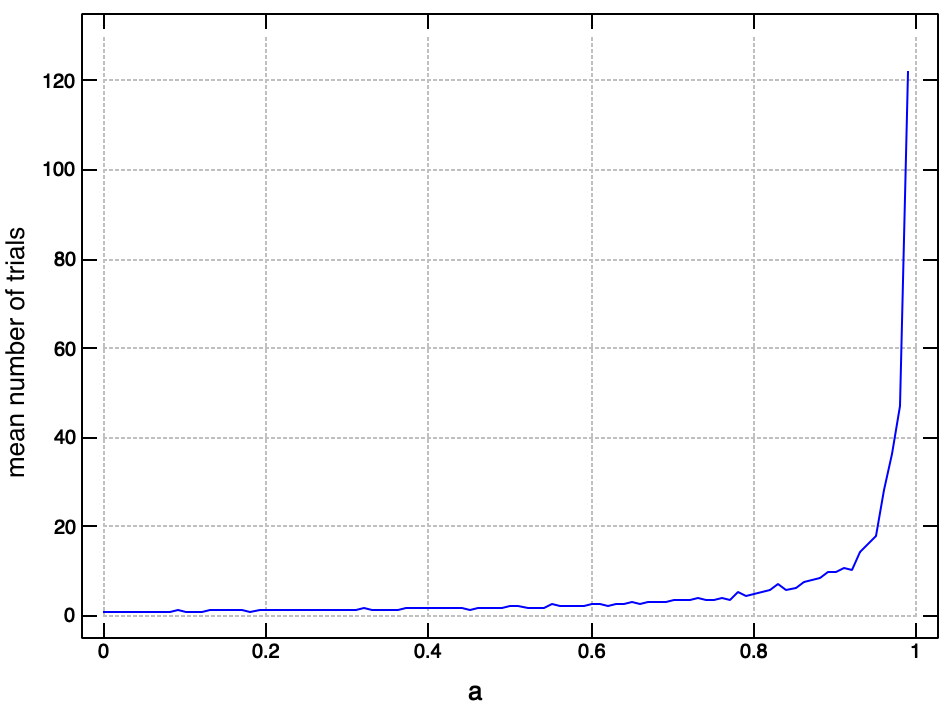
Obviously, though, as \(a\) gets close to 1, the number of trials gets very large, though still finite.
This gives us an idea of what is going on. Obviously, any set of random samples has an empirical mean, which is finite. But the expected value is the asymptotic value of this empirical mean as the number of samples tends to infinity.
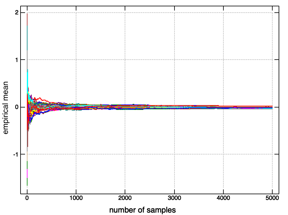
For distributions with an expected value, the empirical mean of such samples will fairly rapidly converge to this true value (the law of large numbers). For instance, if we draw a large number of samples from a standard normal, and plot the running average as we add more samples, we see it converges rapidly to the expected value of \(0\).
What happens if we plot this for a distribution without a mean, like our number of trials above?
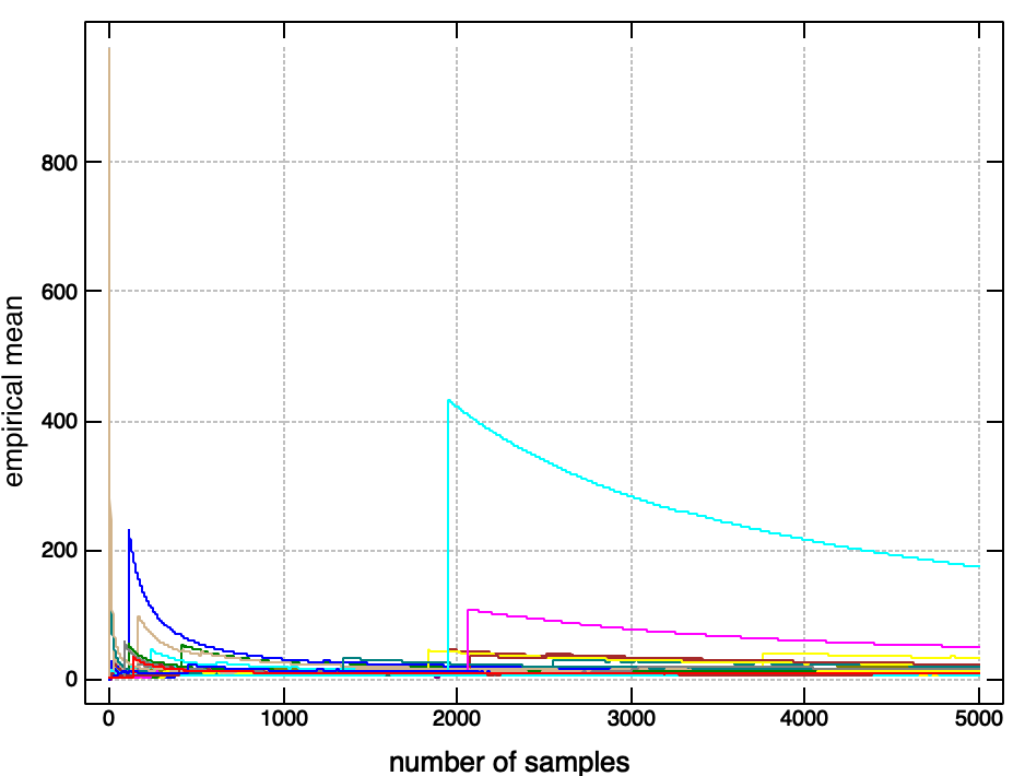
Unlike for a distribution with an expected value, where the fluctuations in the running average are quickly damped down and the running average converges rapidly to the expected value, we see that the running average here is dominated by spikes and jumps. These jumps are caused by irregular, extremely large values, which occur frequently enough in this distribution to prevent the settling down of the mean, unlike in a more ‘well behaved’ distribution like the normal, where very large or very small values are unlikely enough that they get washed out.
This behaviour persists no matter how many samples we draw -
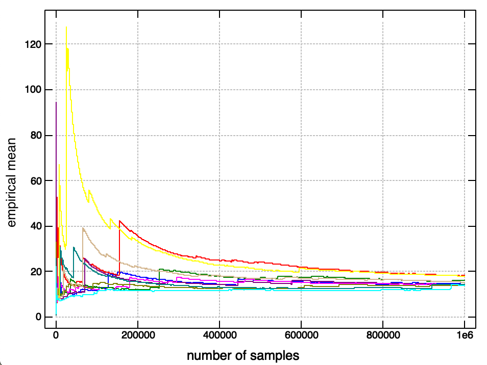
try it yourself! It doesn’t matter how many times you generate these plots, they always look ‘spiky’ in random places. Also notice that the running average tends to slowly increase as we take more samples - this is because the ‘true’ expected value is infinite, but this manifests itself by occasional very large values occuring, so the convergence is irregular.
You can generate plots like this using the following python code;
import numpy as np
from matplotlib import pyplot as plt
n_runs = 5
trials_per_run = 5000
a = np.random.rand(n_runs, trials_per_run)
ev = (1 - a) ** -1
running_avg = np.cumsum(ev, -1) / (1 + np.arange(ev.shape[0]))
plt.plot(running_avg.T)
No discussion of distributions lacking means is complete without a discussion of the Cauchy, the most famous ‘pathological’ distribution
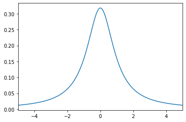
The cauchy distribution is even more pathological than our game here, as it’s mean cannot even be assinged an infinite value. The pdf. of the Cauchy is the innocuous looking
\[ p(x) = \frac{1}{\pi (1 + x^2)} \]
Why can’t the mean be defined? The mean of a random variable is given by the integral
\[ \mathbb{E}[x] = \int_\infty^\infty x p(x) dx \]
for the cauchy, we can compute this indefinite integral fairly easily by substituting \(u = 1 + x^2\)
\[ \begin{aligned} \int x p(x) dx &= \int \frac{x}{\pi (1 + x^2)} dx \\ &= \frac{1}{2\pi} \int \frac{1}{u} du \\ &= \frac{1}{2\pi} \log (1 + x^2) \end{aligned} \]
The issue with this is that for well defined integrals, we must have that for any a
\[ \int^{-\infty}_\infty f(x) dx = \int_{-\infty}^a f(x) dx + \int_a^\infty f(x) dx \]
But for the Cauchy, we can easily see that for \(a=0\),
\[ \begin{aligned} \int^{-\infty}_\infty f(x) dx &= \int_{-\infty}^0 f(x) dx + \int_0^\infty f(x) dx \\ &= -(\int_0^\infty f(x) dx) + \int_0^\infty f(x) dx \\ &= -\infty + \infty \\ \end{aligned} \]
So we can’t consistently assign even an infinite value to this integral.
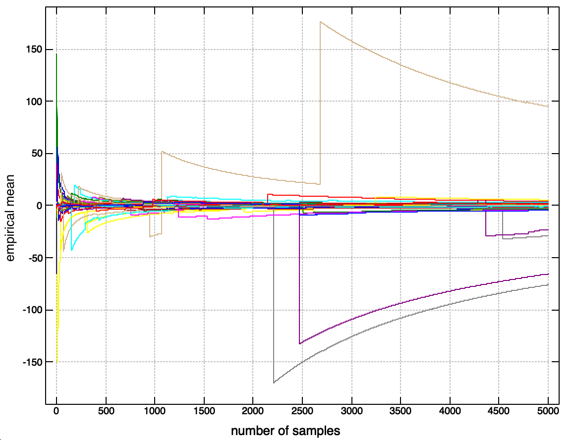
If we visualise the running sample means from the Cauchy, then it has a similar ‘jumpy’ behaviour to the samples from this game, but with no particular preferred direction (wheras the number of runs for the game gradually creeps upwards as we increase the number of samples).
The behaviour of other undefined or infinite moments (like infinite or undefined variance) is intuitively similar to this - the sample variance will have this ‘spiky’ or ‘jumpy’ property, such that no finite sample gives a good estimate of the behaviour of future samples.
Such distributions are probably more common in reality than we would like to admit - many real world phenomena, like market prices, the popularity of music or films, or posts on social media, appear to follow distributions that have the kind of heavy tails that lead to undefined moments.