The following post is a slightly modified version of some notes I made for an internal reading group at Oxford. I actually gave the tutorial ages ago, but I finally got around to cleaning it up and putting it online.

Introduction

In brief, information geometry is the study of the geometrical structure of families of probability distributions. The field thus brings together statistics, information theory and differential geometry, revealing some fascinating and unexpected connections between them. This tutorial attempts to fit a flavour of a fairly technical and abstract field into a brief tutorial that assumes no knowledge of differential geometry. Therefore, I have chosen intuition over rigour whenever I felt it appropriate, for which I make no apologies, and only introduced the absolute minimum of background. I skip over a lot of very interesting things to try to get to the information metric as quickly as possible. There is a list of further reading in the conclusion for those who are interested.

Background - differential geometry

Manifolds

The geometrical space that we are most familiar with is Euclidean or ‘flat’ space \(\mathbb{R}^n\), with the Euclidean distance metric

\[\begin{aligned} d(x, y) = (\Sigma_{i=1}^{n} (y^i - x^i)^2)^{1/2}\end{aligned}\]

A manifold \(\mathcal{M}\) is a space which is locally flat. To be more precise, let us first define or revise some concepts from topology.

A topological space \(X\) is defined by a set of points \(x \in X\) and a set of subsets of \(X\) called neighbourhoods \(N(x)\) for each point. The neighbourhoods obey some axioms which allow a consistent concept of locality. These are that

1. if \(U\) is a neighbourhood of \(x\) (\(U \in N(x)\)), then \(x \in U\)

2. if \(V \subset X\) and \(U \subset V\), and \(U\) is a neighbourhood of \(x\), then \(V\) is also a neighbourhood of \(x\)

3. The intersection of two neighbourhoods of \(x\) is also a neighbourhood of \(x\)

4. Any neighbourhood \(U\) of \(x\) includes a neighbourhood \(V\) of \(x\), such that \(U\) is a neighbourhood of all points in \(V\).

The details of this aren’t really critical here, but basically these axioms create a logically consistent concept of points being ’near each other’ (sharing a neighbourhood) without introducing a distance. I only mention it for completeness because some of the following definitions use it, but you can understand everything that follows if you only have a hand-wavey concept of what a topological space is.

A function \(f : X \to Y\) between two topological spaces is a homeomorphism if

1. \(f\) is a bijection (one to one and onto)

2. \(f\) is continuous

3. the inverse function \(f^{-1}\) is also continuous

If such a function exists between two spaces \(X\) and \(Y\), we say that \(X\) and \(Y\) are homeomorphic)

The bijectivity means we can associate each point in \(X\) with a unique counterpart in \(Y\). The continuity means that we preserve the topological structure around each point - if \(x\) and \(x'\) share a neighbourhood in \(X\), their counterparts \(f(x), f(x')\) are also neighbours in \(Y\). And the continuity of the inverse means that this holds both ways. So a homeomorphism means that we can regard \(X\) and \(Y\) as topologically equivalent.

A topological space \(\mathcal{M}\) is a manifold if for all points \(x \in \mathcal{M}\), there is a neighbourhood \(U\) of \(x\) and some integer \(n\) such that \(U\) is homeomorphic to a subset of \(\mathbb{R}^n\). The smallest such \(n\) is called the dimension of the manifold.

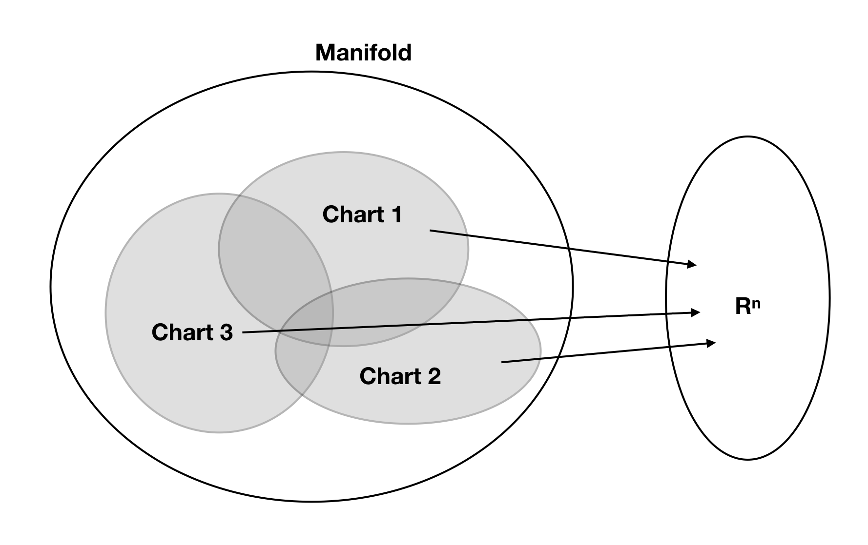
This is saying that there is a region around every point on the manifold that can be treated as being Euclidean. This is what it means for a manifold to be “locally flat” - wherever you are on the manifold, there is at least a small neighbourhood around you that is homeomorphic to flat space. If \(U\) is an open subset of \(\mathcal{M}\), then a homeomorphism \(\kappa : U \to \kappa(U) \subset \mathbb{R}^n\) (which we know exists at every point from the definition above) is called a chart. The chart can be thought of as a local coordinate system that associates a unique set of \(n\) real numbers to each point in a neighbourhood on the manifold. A manifold cannot necessarily be described by only one chart, and there may be several possible valid charts for a given region of the manifold.

Let \(A = \{\kappa_i : U_i \to \kappa_i(U_i) \subset \mathbb{R}^n, U_i \subset \mathcal{M}, i = 1,2,3,...\}\) be a collection of charts on open subsets of \(\mathcal{M}\). We say \(A\) is an atlas if the subsets cover the manifold, that is if \(\bigcup_i U_i = \mathcal{M}\). In addition, we call the functions \(\phi_{ij} = \kappa_i \circ \kappa_j^{-1} : \kappa_j(U_i \cap U_j) \to \kappa_i(U_i \cap U_j)\) the transition maps of the atlas.

An atlas allows us to assign at least one set of coordinates in \(\mathbb{R}^n\) to every point on the manifold. The transition maps allow you to convert between different coordinate systems as defined by different charts in regions where more than one chart is valid . See the figure for a schematic illustration.

An obvious example of a non-trivial manifold is the sphere \(S^2\). It can be shown that there is no chart \(\kappa\) that assigns coordinates to the entire two sphere without degeneracy. The obvious choice of spherical coordinates \(\kappa(p) = (\theta,\phi)\) (latitude and longitude) is not a homeomorphism to Euclidean space over the whole sphere because it is degenerate at the pole (where \(\phi\) could be \(0\) or \(\pi\)) and at the prime meridian (where \(\theta\) could be 0 or \(2\pi\)) which means it cannot be one-to-one. To make this a homeomorphism, we will need to restrict the mapping to exclude these problematic points, and use (at least) two coordinate systems relative to two different poles to cover the whole sphere. An intuitive way to think about this is to say that if you make a cut in a balloon, you can always stretch it out to cover a flat plane, but you need to make a cut. In order to put the balloon back together again, you would need at least two flattened bits of balloon to cover up the hole.

A differentiable manifold has a small amount of additional structure:

A manifold is a differentiable manifold if it has an atlas whose transition maps are all (infinitely) differentiable.

This additional requirement guarantees that we can do calculus in a meaningful way. It implies that a function that is differentiable in one chart is also differentiable in all the others that apply, so it makes sense to speak about differential structures being on the manifold rather than just relative to a particular coordinate system.

In information geometry, we will be concerned with the geometry of statistical manifolds, where every point \(p \in \mathcal{M}\) on the manifold corresponds to a probability distribution over some other domain \(\mathcal{X}\). It is perhaps less obvious at this point than in the previous example what exactly this means, but we can talk about a very simple example already - consider the manifold formed by the family of one dimensional normal distributions. The coordinate systems defined by charts on the manifold correspond to parameterizations of the distribution - for example, one possible chart is \(\kappa(p) = \mu_p, \sigma_p\) that maps distributions to their mean and standard deviation. Another is \(\kappa(p) = \mu_p, \lambda_p\), where \(\lambda\) is the precision parameter. We are interested in the geometry of the underlying space mapped by these parameters. Note that while it will be convenient to confuse a point with its coordinates, they are not the same thing - as the example above shows, a point can have several different coordinate representations, and the choice does not affect the underlying geometry.

While the distinction between the coordinates of a point on a manifold under a particular chart and the geometric object itself is important to keep in mind, in practice we shall be fairly loose with the difference from here on out, and will conflate a point on the manifold with its coordinate representation fairly freely. As we know the manifold has an atlas, for any point \(p\) we can introduce a coordinate representation \(x^a\), where it is understood that the index \(a\) runs from one to \(n\), and we can always choose to work with the co-ordinate representation. Conceptually, a coordinate system is one of the charts, a function that maps points on the manifold into \(\mathbb{R}^n\).¹

We can then proceed to define curves on the manifold by parametric equations in a particular coordinate system

\[\begin{aligned} x^a = x^a(u)\end{aligned}\]

where \(u\) is a parameter that varies along the curve, and \(x^a(u)\) are functions of \(u\). Surfaces and higher dimensional subspaces can be defined similarly by using multiple parameters \(x^a = x^a(u^1,u^2,u^3,...u^n)\).

Covectors, contravectors and tensors

We mentioned above that there may be many valid charts at a particular point \(x\), defining different choices of coordinate systems. It is important, therefore, to see how quantities defined on the manifold behave as we go from one chart to another. Consider changing from the old coordinates \(x^a\) to new coordinates \(x'^a\). The appropriate transition map provides us with a (differentiable) function

\[\begin{aligned} x'^a = \phi^a(x^1, x^2,... x^n)\end{aligned}\]

which we can write more concisely simply as \(x'^a = x'^a(x)\). Differentiating with respect to the original coordinates \(x^b\) gives the Jacobian of the transformation

\[\begin{aligned} \frac{\partial x'^a}{\partial x^b}\end{aligned}\]

The total differential is \[\begin{aligned} dx'^a = \frac{\partial x'^a}{\partial x^b} dx^b\end{aligned}\]

Note that we are using the Einstein summation notation here, where a repeated index in an expression like the one above implies a sum over that index. Indices which occur on both sides of the equation are ‘free’, and can range from \(1\) to \(n\). For example, the Jacobian above has two free indices, and so represents an object with \(n^2\) parameters. In a fixed basis, this corresponds to a matrix.

We can now begin to introduce fields that live on the manifold, and start to talk about how they behave. The simplest object is a scalar field which associates a real number to each point on the manifold. Clearly a scalar field \(\psi\) has the uninteresting transformation behaviour \(\psi(x^a) = \psi(x'^a)\) under a change of coordinates.

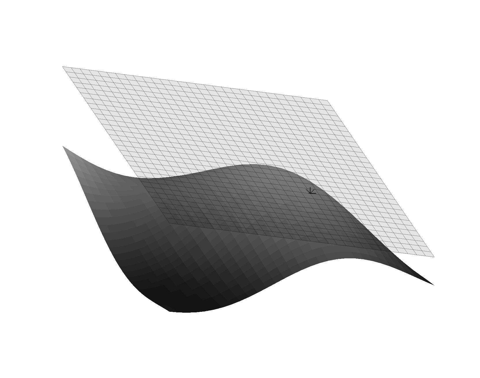
More complex structures are harder to define. For example, in ordinary geometry we are used to thinking of vectors as being the straight line segment connecting two points in space. However, this doesn’t make sense on a manifold, as in general there is no notion of a ‘straight’ line segment in a curved space. Instead, we can define vectors as tangents to a curve at a particular point on the manifold. For a curve \(x^a(u)\), with \(u\) chosen so that \(u=0\) at a point \(p\) on the manifold, we can define the vector \(X^a = \frac{\partial x^a}{\partial u} \rvert_{u=0}\)². It is important to note that this definition is local to the point \(p\) - these vectors do not live on the manifold itself, since they are Euclidean and the manifold is not. The space of possible tangent vectors at a point \(p\) is called the tangent space at \(p\) (see figure ). We can make this more familiar by considering the curves are aligned with the coordinates in a particular chart, that is \(x^a(t_b) = x^a(0) + t \delta^a_b\) where \(\delta_a^b\) is the Kronecker delta, which is \(1\) if \(a = b\) and zero otherwise. The gradients of curves of this type can be used to define a basis set of unit vectors \(\hat{e}^a\) whose representation in a coordinate frame is

\[\begin{aligned} \hat{e}^1 = (1,0,0,0...), \hat{e}^2 = (0,1,0,0...),... \hat{e}^n = (...,0, 1)\end{aligned}\]

These vectors span the tangent space, forming a Cartesian basis. We can then think of the representation of the vector in a \(X^a\) in a particular basis as meaning a linear combination of the basis vectors of that coordinate system \(X^1 \hat{e}^1 + X^2 \hat{e}^2 ...\).

By applying the chain rule, its easy to see that under a change of coordinates at \(p\), the coordinate representation of a vector of this kind transforms as

\[\begin{aligned} X'^a &= \left. \frac{\partial x'^a}{\partial u} \right \rvert_{u=0} \\ &= \left. \frac{\partial x'^a}{\partial x^b} \frac{\partial x^b } {\partial u} \right \rvert_{u=0} \\ &= \frac{\partial x'^a}{\partial x^b} X^b\end{aligned}\]

In general, we will say that

A contravariant vector or contravariant tensor of rank 1 is a quantity, written \(X^a\) in the basis \(x^a\), which transforms under a change of basis as \(X'^a = \frac{\partial x'^a}{\partial x^b} X^b\)

More generally, we can also define contravariant objects of higher rank. For example, a contravariant tensor of rank two transforms as

\[\begin{aligned} X'^{ab} = \frac{\partial x'^a}{\partial x^c} \frac{\partial x'^b}{\partial x^d} X^{cd}\end{aligned}\]

Due to their alignment with common intuitions, we sometimes refer to contravariant vectors as simply vectors.

However, not all vector-like objects transform in this way. Consider a continuous and differentiable scalar field \(\psi(x^a)\) on the manifold. Is the object \(\frac{\partial \psi}{\partial x^a}\) a vector? It has \(n\) coefficients like a vector, but its transformation rule is different. We can write

\[\begin{aligned} \psi = \psi(x^a(x'^b))\end{aligned}\]

considering \(x^a\) as a function of the coordinates of a different frame \(x'^b\). Then, the chain rule gives, after some re-arranging

\[\begin{aligned} \frac{\partial \psi}{\partial x'^a} = \frac{\partial x^b }{\partial x'^a} \frac{\partial \psi}{\partial x^b} \end{aligned}\]

Note that this transforms with the inverse Jacobian, the opposite way to a contra-vector.

A covariant vector or covariant tensor of rank 1 is a quantity, written \(X_a\) in the basis \(x^a\), which transforms under a change of basis as \(X'_a = \frac{\partial x^a}{\partial x'^b} X_b\)

As before, we can generalise this to covariant tensors of higher rank, or tensors of mixed rank. Contravariant indices are written as upper indices, while covariant ones are lower, so \(X^{ab}_{cde}\) has two contra and three covariant rank. More concisely we say it has rank \((2,3)\).

A contravariant vector transforms with the Jacobian of the transformation, while a covector transforms with the inverse Jacobian. While this is not normally stressed, there are some everyday examples you may be more familiar with

The position vector of a point in \(\mathbb{R}^n\) is a contravariant vector

Let \(S\) be a surface in \(\mathbb{R}^3\) parameterised by \(F(x_1,x_2,x_3) = 0\) for some scalar function \(F\). Then the surface normal is given by the gradient \(\nabla F\), or in our notation \(n_a = \frac{\partial F}{\partial x^a}\). The surface normal is the gradient of a scalar field and therefore a covector. It thus transforms with the inverse Jacobian, a fact well known in computer graphics.

The stress in a body can be expressed as a rank two contravariant tensor, \(\sigma^{ab}\). This is defined in such a way that the matrix product of the stress tensor with a surface normal \(n_a\) gives the force \(T^a\) due to the stress across that surface, which is a vector - \(T^a = \sigma^{ab} n_b\).

Distances and the metric

The above defined all vectors, tensors etc. in the tangent space of the manifold at a particular point. So far though, vectors at different points live in different spaces, and we cannot really do a whole lot with them. So far we cannot even define the length of a vector. We might be tempted to use the formula \(\sqrt{\delta_{ab} X^a X^b}\). But it’s easy to check that this is not a scalar in its transformation behaviour, and so is not even a suitable way to compare the size of vectors in the same tangent space.

A metric is a tensor field that induces an inner product on the tangent space at each point on the manifold. In order that the inner product be a scalar, we require that the metric tensor has covariant rank two. Then, for a metric \(g_{ab}\), we can define the inner product between two vector fields \(X\) and \(Y\) as

\[\begin{aligned} \langle X, Y \rangle := g_{ab} X^a Y^b\end{aligned}\]

It is easy to check that this is a scalar. This definition also means that we require \(g_{ab}\) to be symmetric, in order to satisfy the basic property of the inner product that \(\langle X, Y \rangle = \langle Y, X \rangle\)

The metric allows us to define the length of curves on the manifold. For a parameterised curve \(x^a(u)\), the length of an infinitesimal displacement \(dx^a\) is now given by the metric

\[\begin{aligned} dl^2 = g_{ab} dx^a dx^b\end{aligned}\]

then, using the chain rule, we can define the length of a curve as the integral of this line element

\[\begin{aligned} l = \int_{u_1}^{u_2} dl = \int_{u_1}^{u_2} \left( g_{ab} \frac{\partial x^a}{\partial u} \frac{\partial x^b}{\partial u} \right ) ^{\frac{1}{2}} du\end{aligned}\]

Similarly, we can define the volume element of sub-manifolds in terms of the metric as

\[\begin{aligned} dV_n = \sqrt{g} d^nu\end{aligned}\]

where \(g\) is the determinant of the metric \(g_{ab}\).

If \(g\) is non zero, then it follows that there exists a \(g^{ab}\) such that \[\begin{aligned} g^{ab}g_{ab} = \delta^a_b\end{aligned}\] which is called the inverse of the metric. This can be used to ‘raise and lower’ indices, transforming contravectors into a covariant representation and vice versa as follows

\[\begin{aligned} X^a = g^{ab} X_b \\ X_a = g_{ab} X^b\end{aligned}\]

On a manifold with a metric, therefore, we can regard these as being different representations of the same object. ³

In 3d Euclidean space with Cartesian coordinates, the metric is just the identity matrix. In polar coordinates, the line element is \(dl^2 = dr^2 + r^2 d\theta^2 + r^2 \sin^2 \theta d\phi^2\), and the corresponding metric is

\[\begin{aligned} \begin{bmatrix} 1 & 0 & 0 \\ 0 & r^2 & 0 \\ 0 & 0 & r^2 \sin \theta^2 \end{bmatrix}\end{aligned}\]

Note that even a flat space can have a non-trivial metric in a certain coordinates.

In the flat space time of special relativity, the metric of 4-space is \[\begin{aligned} \begin{bmatrix} -1 & 0 & 0 & 0 \\ 0 & 1 & 0 & 0\\ 0 & 0 & 1 & 0 \\ 0 & 0 & 0 & 1 \\ \end{bmatrix}\end{aligned}\] in Cartesian coordinates where the first coordinate is time, and the remaining three are spatial. The opposite sign convention is also used.

In general, any tensor field of covariant rank two can be used to define a metric. In many applications, for example in classical mechanics, the form of the metric is given a priori, while in general relativity the metric of spacetime is the primary object of study (Einstein’s equations, roughly speaking, relate the dynamics of the metric tensor field to the distribution of mass as given by the stress-energy tensor). In general though, mathematically, the metric tensor is arbitrary - any symmetric rank two tensor will do. For the case of statistical manifolds, we might expect there would be many valid metrics we may choose, as there are many ways of defining a divergence between probability distributions. Remarkably however, as we shall see, the statistical manifolds of information geometry turn out to have a uniquely appropriate metric.

Information Geometry

We have now covered enough basic concepts of differential geometry to begin to discuss information geometry. We recall the definition that was mentioned in the introduction

A statistical manifold is a manifold \(\mathcal{M}\) where each point \(p \in \mathcal{M}\) corresponds to a probability distribution \(p(x)\) over some other domain \(\mathcal{X}\)

As mentioned, the statistical structure of these manifolds leads to a unique natural metric. We will attempt to introduce this metric, motivate its derivation, then look at two applications - uniform priors and optimisation.

The information metric

We wish to find a suitable metric tensor at a point \(\theta^a\) on a statistical manifold⁴. Recall that each point \(\theta^a\) corresponds to one of a family of probability distributions \(p(x \mid \theta)\). When we ask for a metric, we are essentially looking for a notion of the distance between a distribution \(p(x \mid \theta)\) and one defined by an infinitesimal perturbation to the parameters, \(p(x \mid \theta + d\theta^a)\). Note that we mean by writing \(\theta\) without an index that the function depends on the whole vector, rather than just one coordinate.

The information metric from distinguishability

There are several ways to derive the information metric. First, we will go over an intuitive one based on distinguishability. Consider the relative difference

\[\begin{aligned} \Delta &= \frac{p(x \mid \theta + d\theta^a) - p(x \mid \theta)}{p(x \mid \theta)} \\ &= \frac{\frac{\partial p(x \mid \theta)}{\partial \theta^a } d\theta^a}{p(x \mid \theta)}\\ &= \frac{\partial \log p(x \mid \theta)}{\partial \theta^a } d\theta^a\end{aligned}\]

The relative difference depends on \(x\), which is a random variable. It does not make much sense to have our geometry be random, so we can consider the expected value of this quantity. However, this vanishes identically

\[\begin{aligned} \mathbb{E}[\Delta] &= \int dx \, p(x\mid \theta) \frac{\partial \log p(x \mid \theta)}{\partial \theta^a } d\theta^a \\ &= d\theta^a \frac{\partial}{\partial \theta^a } \int dx \, p(x \mid \theta) \\ &= 0\end{aligned}\]

so it is not so useful. Instead, we can consider the variance

\[\begin{aligned} \mathbb{E}[\Delta^2] &= \int dx \, p(x\mid \theta) \frac{\partial \log p(x \mid \theta)}{\partial \theta^a } \frac{\partial \log p(x \mid \theta)}{\partial \theta^b } d\theta^a d\theta^b\\\end{aligned}\]

as a measure of the infinitesimal difference between the two distributions, so we could say \(dl^2 = \mathbb{E}[\Delta^2]\) between the points \(\theta^a\) and \(\theta^a + d\theta^a\) on the manifold. Comparing to the formula for the line element

\[\begin{aligned} dl^2 = g_{ab} d\theta^a d\theta^b\end{aligned}\]

this suggests introducing the metric

\[\begin{aligned} g_{ab} :&= \int dx \, p(x\mid \theta) \frac{\partial \log p(x \mid \theta)}{\partial \theta^a } \frac{\partial \log p(x \mid \theta)}{\partial \theta^b } \\\end{aligned}\]

This is none other than the Fisher information, which measures how much information an observation of the random variable \(X\) carries about the parameter \(\theta\) on average if \(x \sim p(x \mid \theta)\). It is easy to check that this quantity is a tensor of covariant rank two, as claimed.

The information metric from the relative entropy

The above procedure may seem slightly arbitrary. To convince you of the generality of this metric, let us derive it in another way. An alternative way to characterise the difference between two distributions is the relative entropy

\[\begin{aligned} D(\theta', \theta) = - \int dx\, p(x \mid \theta') \log \frac{ p(x \mid \theta)}{p(x \mid \theta')}\end{aligned}\]

which measures the information lost if we replace the distribution defined by \(\theta'\) with the one defined by \(\theta\). In information theoretic terms, it is the expected extra number of bits of information needed to encode samples from \(p(x\mid \theta')\) using an optimal code for \(p(x\mid \theta)\) instead of the optimal code for \(\theta'\). This is a natural way to quantify a divergence between probability distributions, but it does not in general define a proper distance (for example, it is not symmetrical).

Let us see how this behaves for infinitesimal changes in \(\theta\), that is, \(\theta'= \theta + d\theta\) for fixed \(\theta\). Since we are considering small changes, we can Taylor expand around \(\theta\). Recall that the relative entropy is strictly greater than zero, with equality only if \(\theta = \theta'\). This means that the zeroth and first order term in the Taylor expansion are zero, since this is a minimum of \(D(\cdot,\theta)\), which gives us

\[\begin{aligned} D(\theta + d\theta, \theta) = \frac{1}{2} \left.\frac{ \partial^2 D(\theta',\theta)}{\partial \theta'^a \partial \theta'^b } \right\rvert_{\theta' = \theta}d\theta^a d\theta^b\end{aligned}\]

where we neglect higher order terms since we are considering infinitesimal displacement. This suggests setting the distance element as

\[\begin{aligned} dl^2 = D(\theta + d\theta, \theta) = \frac{1}{2} \left. \frac{ \partial^2 D(\theta',\theta)}{\partial \theta'^a \partial \theta'^b} \right \rvert_{\theta' = \theta} d\theta^a d\theta^b \\\end{aligned}\]

We can evaluate the second derivative as

\[\begin{aligned} \frac{ \partial^2 D(\theta',\theta)}{\partial \theta'^a \partial \theta'^b} &= \frac{\partial}{\partial \theta'^a} \int dx\, [\log \frac{p(x \mid \theta')}{p(x\mid \theta)}+ 1] \frac{\partial p(x\mid\theta')}{\partial \theta'^b} \\ &= \int dx\, \left[ \frac{\partial \log p(x \mid \theta')}{\partial \theta'^a} \frac{\partial p(x\mid \theta')}{\partial \theta^b} + [\log \frac{p(x \mid \theta')}{p(x\mid \theta)}+ 1] \frac{\partial^2 p(x\mid\theta')}{\partial \theta'^b \partial \theta^a} \right]\end{aligned}\]

Evaluating this at \(\theta' = \theta\), the second term vanishes because

\[\begin{aligned} \int \frac{\partial^2 p(x\mid\theta')}{\partial \theta'^b \partial \theta^a} dx = \frac{\partial^2 }{\partial \theta'^b \partial \theta^a} \int p(x\mid\theta') dx = \frac{\partial^2 }{\partial \theta'^b \partial \theta^a} 1 = 0\end{aligned}\]

and then using that \(\frac{\partial f(x)}{\partial x} = \frac{\frac{\partial f(x)}{\partial x}}{f(x)} f(x) = \frac{ \partial \log f(x)}{\partial x} f(x)\), we obtain that the metric induced by this is

\[\begin{aligned} dl^2 &= D(\theta + d\theta, \theta) = \frac{1}{2} \left. \frac{ \partial^2 D(\theta',\theta)}{\partial \theta'^a \partial \theta'^b} \right \rvert_{\theta' = \theta} d\theta^a d\theta^b \\ &= \frac{1}{2} \int dx \, p(x\mid \theta) \frac{\partial \log p(x \mid \theta)}{\partial \theta^a } \frac{\partial \log p(x \mid \theta)}{\partial \theta^b }\end{aligned}\]

which is, up to an unimportant scaling factor, the Fisher information again.

The uniqueness of the metric

The above demonstrate two motivations that yield the same metric, and I hope that this is enough to persuade you that the information metric is not just a natural choice, but one with surprising generality. Indeed, there are many other ways to arrive at it - I showed the derivation for the KL divergence, but any other \(f\) divergence would have given the same result. It can in fact be shown that the information metric is unique, in the sense that up to a constant factor, it is the only Riemannian metric⁵that is consistent with the fact that points on the manifold correspond to probability distributions. This means that statistical manifolds, purely by virtue of mapping to distributions, do have an intrinsic non-trivial geometry.

The key premise of the argument is information monotonicity. This is a principle about how any measure of divergence, or difference, between probability distributions should behave under ’coarsening’ of our knowledge. Consider the distribution over the faces of a fair dice. We can think about the distribution we get by applying a deterministic function of the outcome space \({1..6}\), that is, \(P(f(x))\). This mapping could be invertible, in which case we don’t really change anything about the distribution - for example, we could have \(f(x) = 2x\). Or it could lose information - for example, a function which is one if the dice roll is even and zero otherwise. The principle of information monotonicity says if we take a divergence measure between \(p_a(x)\) and \(p_b(x)\), then compare it to the divergence between the corresponding distributions over the transformed variable \(p_a(f(x))\) and \(p_b(f(x))\), then the divergence has to be less than or equal the divergence on the original distributions, that is, if the divergence measure is \(D\), that \(D[p_a(x), p_b(x)] \ge D[p_a(f(x)), p_b(f(x))] \forall f\).

If we consider two distributions over the faces of the dice, it’s obvious that doubling the dice score doesn’t affect how easy it is to tell the distributions apart, whereas only telling you the dice is even or odd may make it much harder. What I can’t do is make it easier to tell the distributions apart just by applying some function to draws.

So if we want our measure of divergence to describe statistical difference in any sensible way, we want it to obey this property.

Because this needs to hold for any function \(f\) whatsoever, it’s actually quite a strong constraint on our choice of divergence. I won’t give the full proof here because it’s quite long and a bit technical, but the upshot is that it can be shown that any distance (or divergence) between probability distributions that obeys the information monotonicity principle wouldgive rise to the Fisher metric, up to a constant, by considering the Hessian of the divergence as we did for the KL above.

Uniform Priors

One immediate consequence of statistical manifolds having an intrinsic natural metric is in the design of uninformative prior distributions in Bayesian inference. We could simply use a (possibly improper) prior that assigns uniform mass to all parameter values. But what this prior means depends on the choice of parameterisation - For a Gaussian, for example, a uniform distribution over the precision is a very different distribution to a uniform distribution over the variance, which is different again to a uniform distribution over the standard deviation. Is there such a thing as an objectively uninformative prior? The information metric can provide an answer. Recall that the volume element on a manifold is defined in terms of the metric. Therefore, we can ask for a probability distribution that assigns equal probability to equal volumes of the statistical manifold. Since the only unique metric on the statistical manifold is the Fisher information \(g_{ab}\), this leads to Jeffrey’s prior

\[\begin{aligned} p(\theta) \propto \sqrt{g} \end{aligned}\]

or in more familiar notation,

\[\begin{aligned} p(\theta) \propto \sqrt{\det \mathcal{I}(\theta)} \end{aligned}\]

where \(\mathcal{I}\) is the Fisher information matrix of the parameter vector. Jeffrey’s priors are often improper for real valued parameters, but they are objectively uninformative in a parameterisation independent sense.

Optimisation & the natural gradient

It is a fairly common in statistics to optimise over a family of probability distributions, for example to find the parameters \(\theta\) that maximise the likelihood of some data. A popular method is to use gradient based optimisation to do so. We will now attempt to place gradient descent in the language of differential manifolds. In order to do this, we need to consider continuous paths rather than discrete steps, as adding together points not infinitesimally close is not possible on a manifold.

We can regard the cost function we are trying to minimise (say the negative log likelihood) as a scalar field \(J(\theta^a)\). We want to define a curve \(\theta^a(t)\) that will move to lower \(J\). An obvious way to try to do this is to set the following differential equation for the path of \(\theta^a\)

\[\begin{aligned} \frac{\partial \theta^a}{\partial t} = - \frac{\partial J}{\partial \theta^a}\end{aligned}\]

Unfortunately, this equation makes no geometrical sense. The left hand side, the velocity field, is the tangent to a curve \(\theta^a(t)\) and is therefore a contravectors. But the right hand side is the gradient of a scalar field - a co vector. Since these quantities transform differently under a change of coordinates, we cannot set them equal to each other in a parameterisation-independent way. The fix is to use the inverse metric to ‘raise the indices’ on the other side, giving

\[\begin{aligned} \frac{\partial \theta^a}{\partial t} = - g^{ab} \frac{\partial J}{\partial \theta^b}\end{aligned}\]

which is a well behaved equation. The only way the first version can work is if we assume that the parameters can be treated as Cartesian coordinates in a Euclidean space, in which case the metric is simply the identity. Using standard gradient descent essentially amounts to an assumption, or at least approximation, that this is appropriate. But as we have seen, if the parameters define probability distributions, then the appropriate metric is the Fisher information. This suggests the following modified update rule

\[\begin{aligned} \theta_{t+1} = \theta_t - \eta \mathcal{I}^{-1} \nabla J(\theta)\end{aligned}\]

where, again, \(\mathcal{I}\) is the Fisher matrix of the parameters.

This update rule has the nice property that it is invariant to changes of parameterisation of the distribution. It bears a strong resemblance to Newton’s method, which gives the rule

\[\begin{aligned} \theta_{t+1} = \theta_t - \eta H^{-1} \nabla J(\theta)\end{aligned}\]

where \(H_{ij} = \frac{\partial^2 J}{\partial \theta^i \theta^j}\) is the local Hessian of the parameters. Newton’s method, since the Hessian is also a rank two covariant tensor, is likewise invariant to changes in parameterisation. There is in fact a very close relation between second order methods designed for stochastic optimisation and the natural gradient, a link which is explored in detail in . Like second order methods, natural gradient methods can offer much faster and more reliable convergence than standard gradient descent. Approximations to the natural gradient are a component, for example, of the trust-region policy gradient algorithm .

The natural gradient also suffers from similar computational issues to second order approximations. The Fisher matrix can only be computed in closed form in very simple cases, and the expectation often has to be replaced with empirical sampling. In addition, storing and inverting a matrix of \(N^2\) in the number of parameters is often prohibitive. Nevertheless, various kinds of approximations have been devised that yield a practical, and in some cases very competitive, family of optimisation algorithms.

Conclusion and further reading

I have tried to give a brief introduction to some key ideas in information geometry and some examples of it’s usefulness for practical statistical methods without relying too much on more advanced topics in differential geometry. There is considerably more to study, but it is more technical, and the presentation is often fairly formal and difficult. Examples of things I have not mentioned are characterising the overall curvature of statistical manifolds, and the theory of dual affine connections, partly because these require introducing more geometry than I felt able to do in the scope of this tutorial.

References

1. Ariel Caticha, “The basics of information geometry”, AIP Conference Proceedings, volume 1641,2015

2. Ray D’Inverno, “Introducing Einstein’s Relativity”, 1997, Oxford University Press

3. “A comprehensive introduction to differential geometry”, Michael Spivak,1970, Publish or Perish

4. “Entropic Inference and the Foundations of Physics” (monograph commissioned by the 11th Brazilian Meeting on Bayesian Statistics, Ariel Caticha, http://www.albany.edu/physics/ACaticha-EIFP-book.pdf,2012

5. “Trust region policy optimisation” John Schulman et. al, International Conference on Machine Learning,2015

6. “Why natural gradient?”, Shun-ichi Amari and Scott C Douglas,ICASSP,1998

7. “Revisiting natural gradient for deep networks”, Razvan Pascal and Yoshua Bengio, arXiv:1301.3584,2013

8. “An elementary introduction to information geometry”, Frank Nielsen,arXiv:1808.08271,2018

9. ”A natural policy gradient”, Sham M Kakande,Advances in Neural Information Processing Systems,2002

10. “New insights and perspectives on the natural gradient method”, James Martens,arXiv:1412.1193, 2014

11. “Methods of information geometry”, Shun-ichi Amari and Hiroshi Nagaoka, 2007,American Mathematical Soc.